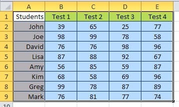
First off, I’ve created a set of student test data for our example. There are eight students with their test scores on four exams. To make this into a chart, you first want to select the entire range of data, including the titles (Test 1, etc).
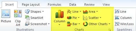
Now that your data is selected as shown above, go ahead and click on the Insert tab on the ribbon interface. A little to the right, you’ll see the Charts section as shown below.
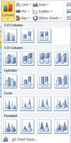
By default, it tries to list out the most common types of charts such as Column, Line, Pie, Bar, Area, and Scatter. If you want a different type of chart, just click on Other Charts. For our example, we will try use a column chart to visualize the data. Click on Column and then select the type of chart you would like. There are many options! Also, don’t worry because if you pick a chart you don’t like, you can easily change to another chart type with just a click of your mouse.
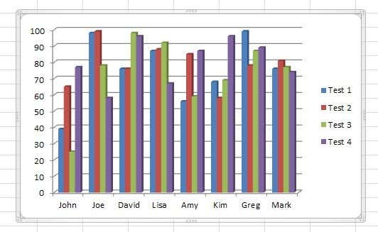
So now Excel will create the chart based on the data and dump it somewhere on your sheet. That’s it! You have created your first graph/chart in Excel and it literally takes just a few minutes. Creating a chart is easy, but what you can do with your chart after making it is what makes Excel such a great tool.
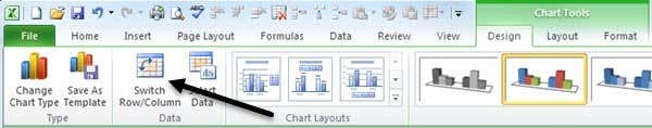
In the above example, I see each person along the X axis and the test scores on the Y axis. Each student has four bars for their respective test scores. That’s great, but what if I wanted to visualize the data in a different way? Well, by default, once the chart is added, you’ll see a new section at the top of the ribbon called Chart Tools with three tabs: Design, Layout and Format. Here you can change everything under the sun when it comes to your new chart.
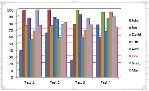
One neat thing you can do is click on Switch Row/Column under Data and the chart will instantly change with the data switched. Now here’s what the chart looks like with the same data, but with X and Y switched.
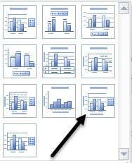
This chart is useful too because now I can see the scores for all the students per exam. It’s very easy to pick out who did the best and who did the worst on each test when the data is displayed like this. Now let’s make our chart a little nicer by adding some titles, etc. An easy way to do this is to click on the little down arrow with a line on top of it under Chart Layouts. Here you’ll see a bunch of different ways we can change the layout.
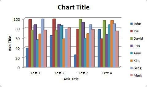
If you pick the one shown above, you chart will now look like this with the additional axis titles added for you. Feel free to choose other layouts just to see how the chart changes. You can always change the layout and it won’t mess up the chart in any way.
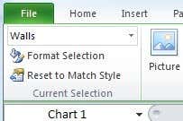
Now just double-click on the text boxes and you can give the X and Y axis a title along with giving the chart a title also. Next let’s move on to the Layout tab under Charts Tools. This is a very important tab because you can tweak pretty much every little detail about your chart here. The best part I like is right on the left part of the ribbon called Current Selection.
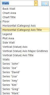
There’s a drop down box that lets you pick any specific part of the chart and then you can click Format Selection to change the settings for just that one part. Here you can see all the different sections you can select:
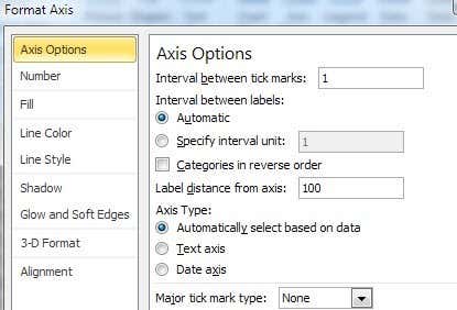
Suppose I click on Horizontal (Category) Axis and then click on Format Selection. I’ll get a dialog window that will let me adjust any and all properties for that object. In this case, I can add shadows, rotate the text, add a background color, etc.
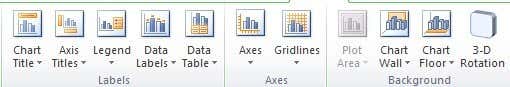
Moving along the ribbon still under Layout, you’ll see a bunch of other options in the Labels, Axes, and Background sections. Go ahead and click on these and try them out to see what kind of effect they have on the chart. You can really customize your chart using these options. Most of the options here basically let you move things to different locations on the chart.
Finally, the Format tab under Chart Tools will let you adjust the formatting on every part of the chart. Again, you can use the Current Selection tool on the left and then change the border styles, font styles, arrangement of objects, etc.
For the fun of it, I added a reflection effect to all the text on the chart and gave the whole chart a 3D effect of coming from the back to the front instead of just flat.
In Excel, you can create far more complicated charts than the one I have shown here, but this tutorial was just to get your feet wet and understand the basics of creating a chart. If you have any questions about the tutorial or you own chart, please leave a comment. Enjoy!